Working with variants in ZonationR

This vignette demonstrates how to explore multiple prioritization scenarios using ZonationR. Users will:

1. Run a baseline prioritization.
2. Modify the marginal loss rule.
3. Apply feature weights.
4. Restrict the analysis to a geographic mask.
5. Include cost considerations.

Following Zonation best practices, analyses are developed incrementally through variants. Each variant modifies specific inputs or settings and is run in its own folder. Folder names are based on key settings used in each scenario. For example, 03_cazmax_w indicates the third variant used the CAZMAX marginal loss rule with feature weights:

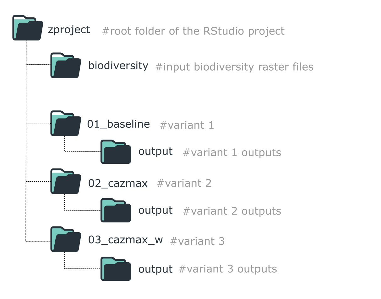
Folder structure for organizing a ZonationR workflow with multiple variants.

This staged workflow keeps each variant isolated, reproducible, and easy to compare. In R, we use withr::with_dir() to temporarily change the working directory for each variant, keeping the project organized while running multiple scenarios.

Setup

# Install 'withr' package if not already installed
if (!requireNamespace("withr", quietly = TRUE)) {
  install.packages("withr")
}

# Load necessary libraries
library(ZonationR)
library(Zonation5RData)
library(withr)

Prepare input data

In this tutorial, we use the Zonation5RData package, which provides GeoTIFF layers for workflows with Zonation and ZonationR. To use the layers in the RStudio project, we first create folders and then copy the raster files from the package.

# Create folders to store the input data
dir.create("biodiversity", showWarnings = FALSE)
dir.create("other_layers", showWarnings = FALSE)

# Get the paths to biodiversity rasters included in the package
files_biod <- zonation5rdata_list("biodiversity", full.names = TRUE)

# Copy the biodiversity rasters to the local biodiversity folder
file.copy(files_biod, "biodiversity", overwrite = TRUE)

# Get the paths to the additional layers included in the package
files_other <- zonation5rdata_list("other_layers", full.names = TRUE)

# Copy these rasters to the local other_layers folder
file.copy(files_other, "other_layers", overwrite = TRUE)

Variant 1

We begin with a baseline prioritization using default settings.

# Run baseline variant in folder 01_baseline
dir.create("01_baseline", showWarnings = FALSE)
withr::with_dir("01_baseline", {
  feature_list(spp_file_dir = "../biodiversity")
  settings_file(feature_list_file = "feature_list.txt")
  command_file(zonation_path = "C:/Program Files (x86)/Zonation5")
  run_command_file(".")
})

Variant 2

In this variant, we change the marginal loss rule to Core-Area Zonation (CAZMAX). CAZMAX aims to always cover high-occurrence locations for all features, even if this comes at the cost of lower average coverage.

# Create the folder
dir.create("02_cazmax", showWarnings = FALSE)

withr::with_dir("02_cazmax", {
  feature_list(spp_file_dir = "../biodiversity")
  settings_file(feature_list_file = "feature_list.txt")
  command_file(zonation_path      = "C:/Program Files (x86)/Zonation5",
               marginal_loss_mode = "CAZMAX" # We edit the marginal loss rule here
  )
  run_command_file(".")
})

Variant 3

We can assign unique weights to features (e.g., species) to increase the priority of areas where those features occur. This allows emphasizing key species or biodiversity features in the prioritization. For this purpose, we use the weight argument in the feature_list() function. To ensure that these weights are applied during analysis, the w flag must also be included in the command_file() call.

For a complete reference of all available analysis flags and their requirements in ZonationR, please see the vignette Analysis flags in ZonationR.

# Create the folder
dir.create("03_cazmax_w", showWarnings = FALSE)

# List files from the folder
spp_files <- list.files("biodiversity", pattern = "\\.tif$", full.names = TRUE)

# Create a weight vector: default weight = 1 for all species
weights <- rep(1, length(spp_files))

# Set higher weights for selected key species
# For example, species 3, 7, and 10 are more important
weights[c(3, 7, 10)] <- 5.0

# Run the prioritization
withr::with_dir("03_cazmax_w", {
  feature_list(spp_file_dir = "../biodiversity",
               weight = weights) # setting weights
  settings_file(feature_list_file = "feature_list.txt")
  command_file(zonation_path = "C:/Program Files (x86)/Zonation5",
               marginal_loss_mode = "CAZMAX",
               flags = "w" # Flag w (use weights)
  )
  run_command_file(".")
})

Variant 4

In this variant, we restrict the prioritization to a subset of European countries. Only areas within the area mask are considered for the ranking process. This approach is useful for focused conservation planning in a defined geographic region.

dir.create("04_cazmax_wa", showWarnings = FALSE)

withr::with_dir("04_cazmax_wa", {
  feature_list(spp_file_dir = "../biodiversity",
               weight = weights)
  settings_file(feature_list_file = "feature_list.txt",
                analysis_area_mask_layer = "../other_layers/area_mask.tif")
  command_file(zonation_path = "C:/Program Files (x86)/Zonation5",
               marginal_loss_mode = "CAZMAX",
               flags = "wa" # Flag a for analysis area mask
  )
  run_command_file(".")
})

Variant 5

In this variant, we include a cost layer using the Global Human Modification (GHM) dataset. Cells with higher human impact are penalized, reducing their priority in the ranking.

dir.create("05_cazmax_waX", showWarnings = FALSE)

withr::with_dir("05_cazmax_waX", {
  feature_list(spp_file_dir = "../biodiversity",
               weight = weights)
  settings_file(feature_list_file = "feature_list.txt",
                analysis_area_mask_layer = "../other_layers/area_mask.tif",
                cost_layer = "../other_layers/gHM_Europe.tif") # We add the cost layer here
  command_file(zonation_path = "C:/Program Files (x86)/Zonation5",
               marginal_loss_mode = "CAZMAX",
               flags = "waX" # using X to activate the cost analysis
  )
  run_command_file(".")
})

Key takeaways

This workflow demonstrated how to construct a variant-based prioritization analysis using ZonationR, with each variant introducing new components to the prioritization setup:

Variant	Description
01	Baseline prioritization using default settings
02	Prioritization with CAZMAX marginal loss rule
03	CAZMAX rule plus feature/species weighting applied
04	CAZMAX with weighting and restricted to a geographic mask
05	CAZMAX with weighting, geographic mask, and cost layer (GHM)

Developing analyses in incremental variants improves transparency, reproducibility, and scenario comparison in spatial conservation planning. To explore the outputs generated by these analyses (e.g., rank maps, performance curves), see the Zonation outputs vignette, which provides guidance on interpreting and visualizing Zonation results.